
UNIVERSIDADE
DO ALGARVE

MANUAL
>>>>>>>>>>
>>>>>>>>>>>>>
>>>>>>>>>>>>>
Nov 2004, Joaquim Luis
email:
download the NEW 0.7 pdf version
Mirone
By
Joaquim Luis
(CIMA - University of Algarve)
Mirone is a Windows MATLAB-based framework tool that allows the display and manipulation of a large number of grid formats trough its interface with the GDAL library. Its main purpose is to provide users with an easy-to-use graphical interface to the more commonly used programs of the GMT package. In addition it offers also a large number of tools that are particularly focused to the fields of geophysics and earth sciences. Among them the user can find tools to do multibeam mission planning, elastic deformation studies, tsunami propagation modeling, IGRF computations and magnetic Parker inversions, Euler rotations and Euler poles computations, plate tectonic reconstructions, seismicity analysis and focal mechanism plotting. The high quality mapping and cartographic capabilities that made GMT known worldwide is guaranteed trough the Mirone’s capability of automatically generating GMT cshell scripts and dos batch files.
As mentioned, Mirone is written using the MATLAB programming language. MATLAB is a very powerful tool for software development. The language is very is easy to learn and contains an endless collection of mathematical functions that highly facilitates the task of writing complicated code, including Graphical Users Interfaces. However, it also suffers from important limitations. Speed and specially memory consumption are the main ones.
To circumvent the above constrains almost all heavy computations involving matrix data are done in Mirone with the help of external code written in C and compiled as mex files. Since those mex files use the scalar programming type and use single precision or short integer variables whenever that is all that is need to not compromise the result accuracy, their memory consumption is reduced to the minimum necessary while the running speed is that of a compiled code.
Before Start
Illustration of the initial GUI state before loading any raster dataset. To load a GMT grid simply hit the folder icon. Loading other formats require selection from the File menu.
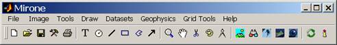
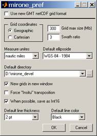
Upon start the user is presented with Mirone in its basic form which is a simple menu bar menus. Activities are initiated by using those menus. Although Mirone comes with pre-defined defaults it is very important that the user understand what they mean and do. The first time the program is used the user is strongly advised to hit the button with hammers icon. That opens the preferences window. The meanings of those settings are as follow:
 ·
“Use new GMT netCDF grid
format”. Starting with GMT version 4.1 a new flavor of GMT
netCDF grids, which are COARS compliant, was introduced. While
this change is transparent to users, the new grid format will no
be recognized by previous GMT versions. If checked new grids
will be written using the new format, otherwise use the old GMT
format. NOTE: this affects only the writing. Upon reading the
grid format is automatically detected
·
“Use new GMT netCDF grid
format”. Starting with GMT version 4.1 a new flavor of GMT
netCDF grids, which are COARS compliant, was introduced. While
this change is transparent to users, the new grid format will no
be recognized by previous GMT versions. If checked new grids
will be written using the new format, otherwise use the old GMT
format. NOTE: this affects only the writing. Upon reading the
grid format is automatically detected
· The grid/image type of coordinates. Select Geographic (default) if you are working with a grid whose coordinates are longitude and latitude. Select Cartesian otherwise. This is an important setting because some operations, like measuring, depend on knowing if we are dealing with geographic or Cartesian coordinates. When a grid is read, Mirone tries to guess what coordinates it has and although it guesses correctly most of times, it may also fail.
· "Grid Max size". In order to do all grid manipulations Mirone stores the original grid in the computer’s memory (regardless of their type they are always stored as single precision). This is the maximum size in Mb that a grid can have and be held on the computer's memory. This doesn't mean that larger grids/images cannot be processed. It only means that if they are larger than this value, they will be re-read from disk whenever necessity demands. It is up to you (based of course on the computer capabilities) to decide on a reasonable value for this parameter. Grid size is computed in the following way: n_rows x n_columns x 4 / (1024*1024). Note: Mirone does most of its heavy computation with external MEX files that use single precision arithmetic's. However, some operations may still be done with MATLAB operators which imply double precision (in this case it takes twice as much memory). When you are using image files, however, this rule does not apply anymore. In fact there is no obvious rule because you may be using compressed or uncompressed images.
· "Swath ratio". When doing a multibeam planning one always has to know the swath width coverage as a function of the water depth. When you start the first track, a question will be made if you accept this value or want to change it. Subsequent tracks won't ask it again, so if you want to change it in the middle of a planning session, you have to come here.
· "Measure unites". When computing distances that's the result is presented in the chosen unit. Available options are: nautical miles, kilometers, meters and user (it means I don't know what are these).
· "Default ellipsoide". Mirone computes distances on an ellipsoidal Earth. Among the various ellipsoids you will also find one for Mars. Don't forget to select this when working with MOLA grids.
· "Working directory". To reduce the cumbersome task of browsing trough the directory tree every time you need to save a file, the program uses a default working directory. You may either write the full path here or press the side button and select one within the selecting window that will open. Besides this mechanism, the program also remembers the last directory used to open a file and will use it as a first guess for the next time you need to open another file.
· "New grids in new window". Many of the possible options involve the computation of a new grid. This parameter controls if the newly computed grid is automatically open in a new Mirone window (if the option is checked) or saved on a disk file. Note that the default mode will also let you save the new grid.
· "Force insitu transposition". This is an option to help importing large grids. Importing grids implies a conversion that uses matrix transposition. This operation is fast if we make a copy of the importing grid. However, this requires twice the grid size on memory. If you do not have enough memory to import a large grid, use this option that do the transposition insitu. That is, it uses only one time the grid size in memory. The price to pay, however, is in speed because it runs about 10 times slower.
· "When possible save as int16 ". Some grids use short ints (2 bytes) to save disk space. Checking this option means that if you save that grid in the GMT format the 2 bytes original density will be retained (otherwise, it will be saved as floats – 4bytes). Useful for example to convert SRTM grids into the GMT format.
· "Default line thickness". Use this default value for drawing lines, circles or other graphical elements.
· "Default line color". Use this default value for drawing lines, circles or other graphical elements (such as text strings).
File menu
·
 New
empty window Opens a new empty
Mirone window from where you can open another file. You can
obtain the same result by clicking on the first icon of Mirone's
Tool bar.
New
empty window Opens a new empty
Mirone window from where you can open another file. You can
obtain the same result by clicking on the first icon of Mirone's
Tool bar.
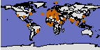
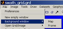
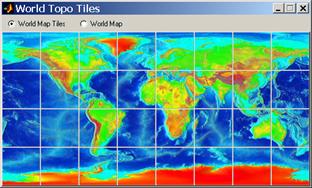
· Background window Allows you to load a background map selectable from those available with the program. You can either select a tile of the world map or the whole world. The selection is carried via a window tool. You can also select a blank map, for which the corner coordinates will be asked.
·
 Open
Grid/Image By default Mirone
automatically detects and reads GMT as well as Surfer 6 or 7
grids. NOTE: generic 2D netCDF grids conforming to the COARDS
convention are also recognized by GMT (and therefore by Mirone),
however, if an error in reading occurs GMT will issue an exit
command that will also shut down Mirone (and Matlab). For other
formats select the type of file you want to open from the
available options. Those options are a large subset of the GDAL
supported formats. Excluded from GDAL formats are those that
deal with satellite images (they are complicated to manipulate
and potentially very big). It is also possible to read MOLA
(Mars grids) files. Surfer 6 and 7 binary grids are detected
automatically. Inside the Digital Elevation you will find
DTED, ESRI BIL, GTOPO30, GeoTIFF DEM, MOLA DEM, SRTM 1, 3 & 30,
USGS DEM, USGS SDTS DEM. The Generic Formats are the
common image formats (png, jpeg, tiff, etc…)
Open
Grid/Image By default Mirone
automatically detects and reads GMT as well as Surfer 6 or 7
grids. NOTE: generic 2D netCDF grids conforming to the COARDS
convention are also recognized by GMT (and therefore by Mirone),
however, if an error in reading occurs GMT will issue an exit
command that will also shut down Mirone (and Matlab). For other
formats select the type of file you want to open from the
available options. Those options are a large subset of the GDAL
supported formats. Excluded from GDAL formats are those that
deal with satellite images (they are complicated to manipulate
and potentially very big). It is also possible to read MOLA
(Mars grids) files. Surfer 6 and 7 binary grids are detected
automatically. Inside the Digital Elevation you will find
DTED, ESRI BIL, GTOPO30, GeoTIFF DEM, MOLA DEM, SRTM 1, 3 & 30,
USGS DEM, USGS SDTS DEM. The Generic Formats are the
common image formats (png, jpeg, tiff, etc…)
·
 Open
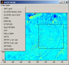
Overview Tool This tool is meant
to be used with very large grids. The selected grid is
sub-sampled, during the reading stage, in order to obtain an
overview of about 200 rows/ columns. This way, arbitrarily large
grids may be previewed, but the quality of the preview will
degrade with grid size. Click on the rectangle icon to draw a
rectangle on the image. Double clicking the rectangle lets you
edit it. A precise control of the rectangle size is available by
a right-click and selecting "rectangle-limits". Selecting "Crop
Grid" extracts the region inside the rectangle at the grid’s
full resolution.
Open
Overview Tool This tool is meant
to be used with very large grids. The selected grid is
sub-sampled, during the reading stage, in order to obtain an
overview of about 200 rows/ columns. This way, arbitrarily large
grids may be previewed, but the quality of the preview will
degrade with grid size. Click on the rectangle icon to draw a
rectangle on the image. Double clicking the rectangle lets you
edit it. A precise control of the rectangle size is available by
a right-click and selecting "rectangle-limits". Selecting "Crop
Grid" extracts the region inside the rectangle at the grid’s
full resolution.
· Open Session Open a previously saved session (see below the Save Session).
· Save Image As… Saves the current display image into one of the common image formats (e.g. jpg, tiff, bmp, etc...). Notice that graphic elements (e.g. lines) are not saved. Only the image is (but see Export).
·
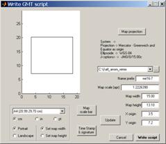 Save
GMT script cshel or dos batch files generation. In this
window it is possible to fine tuning the map details like its
size and position on the page as well as the map projection.
This tool searches systematically all elements and guesses how
they where produced. It than decides what is the best way to
reproduce the display using only GMT commands. For example, if
the image displayed derives from a GMT grid and it was
illuminated with the shading method used by grdgradient
the script lines will generate an illumination grid from the
original GMT grid and use grdimage with the –I option. If
that is not the case then a screen capture is executed and the
image saved as three R,G,B grids. Those three grids are than
utilized by grdimage to rebuild a color image. Line elements are
written on disk and lately used by psxy. However,
coastlines, national borders and rivers or contour lines are not
saved. Instead, appropriate calls to pscoast or
grdcontour are insert into the script. To change the map
size, double click over the rectangle and that click and drag.
Every time you edit the rectangle is necessary to hit the
“Update” button. The script (or the batch file) and the eventual
auxiliary files are written into the directory declared bellow
the Map projection settings. The script (or batch file) is
abundantly commented which makes it easy to educated GMT users
to change it further if they are not fully satisfied with the
code generated result. To run it, just cd to the directory it
was saved and type its name.
Save
GMT script cshel or dos batch files generation. In this
window it is possible to fine tuning the map details like its
size and position on the page as well as the map projection.
This tool searches systematically all elements and guesses how
they where produced. It than decides what is the best way to
reproduce the display using only GMT commands. For example, if
the image displayed derives from a GMT grid and it was
illuminated with the shading method used by grdgradient
the script lines will generate an illumination grid from the
original GMT grid and use grdimage with the –I option. If
that is not the case then a screen capture is executed and the
image saved as three R,G,B grids. Those three grids are than
utilized by grdimage to rebuild a color image. Line elements are
written on disk and lately used by psxy. However,
coastlines, national borders and rivers or contour lines are not
saved. Instead, appropriate calls to pscoast or
grdcontour are insert into the script. To change the map
size, double click over the rectangle and that click and drag.
Every time you edit the rectangle is necessary to hit the
“Update” button. The script (or the batch file) and the eventual
auxiliary files are written into the directory declared bellow
the Map projection settings. The script (or batch file) is
abundantly commented which makes it easy to educated GMT users
to change it further if they are not fully satisfied with the
code generated result. To run it, just cd to the directory it
was saved and type its name.
· Save As GMT grid When you imported a Digital Terrain Model (or whatever function that is represented in the grid) in a format other than the GMT format (e.g. a GTOPO30 file), you can use this option to save that grid as GMT grid (netCDF). Note that you cannot use this option to save an image of any type.
· Save As 3 GMT grids (R,G,B) - Decompose the color image into 3 components, Red, Green & Blue and save each of these components into a GMT grid file. The output name is used as a template to which the _r, _g & _b strings are appended in order to identify the individual color components. This option is extremely useful with GMT4 version, for it will allow transforming any image into GMT grids. You can than (for example) drape satellite images over DTMs, use the alternate illumination algorithms, etc... There are two options on how to save. Image only will save only the image and ignore all graphic elements that may have been added. It will also create grids that have the same number of rows and columns as the original file (be it a grid or an image). Screen capture saves the image, and everything that may have been added to it, by doing a screen capture. The final image size is unknown to me for it's done by an undocumented Matlab function.
· Save As Surfer 6 grid - Saves the current grid (not images) in the Surfer 6 binary grid format. Note, however, that surfer 6 and 7 grids are automatically detected upon reading and will be saved on this format even this option is not selected.
· Save As Encom grid - Saves the current grid in Encom (www.encom.com.au) grid format.
· Save As ESRI .hdr – Saves the current grid in a raw format plus a .hdr header file that makes it suitable to be imported by software that recognize this format.
· Save as GeoTIFF - Saves the current image as a GeoTIFF file. Image only means that only the image is saved (no graphic elements) whereas Screen capture will do what it says capturing also all elements present in the image. Note, the GeoTIFF file size may differ considerably between these two options.
· Save as Fledermaus object - Grids (with what ever they contain) may be saved as .sd IVS objects. These objects may be viewed with the iview3d free Fledermaus viewer. Fledermaus is a fantastic 3D software (probably the best) and has a free viewer that can be downloaded from www.ivs.unb.ca/products/iview3d/. If you have it installed you can either use this option to create a .sd file and separately run it with the viewer or click the icon "eye" in the Tool bar which will do both (but not save the .sd file). Note that large grids produce large .sd files so if you don't have that much RAM (or you want to save the .sd for later use) it may be better to use this save option.
· Save Session - Saves the current state of your work, including all (well, most of all) graphic (drawing) elements into a matlab .mat file. Selecting Open Session resumes the saved session. Very useful for backups. Notice that the grid file is not stored but only the information needed to reconstruct the image. So if the original grid is not found you cannot resume your session. This functionality is not up-to-date with the latest added options (e.g. drawing Euler pole circles) and cannot be used with other images than those derived from GMT grids.
· Export - Do a screen capture and save it into one of the common image formats. This differs from Save Image As where graphic elements (e.g. lines) are not saved. The image size is (un)determined by the same unknown mechanism mentioned in Save As 3 GMT grids (R,G,B)
· Grid/Image -> workspace – This option and the others in this group will only show up in the Matlab running version. It allows exporting variables into the Matlab’s workspace that you can manipulate using the full power of the Matlab engine. Depending on what you are exporting, a different group of variables is generated.
When exporting from a loaded grid the set of variables is: Z an array of doubles containing the grid data; img the image derived from Z; head a 1x10 row vector with [x_min x_max y_min y_max z_min z_max reg x_inc y_inc grd_format] ; X & Y row vectors with the grid’s x & y coordinates; FigHand the figure handle and is_grid which will be 1 to indicate that we have a grid.
When exporting from a loaded image, the variables are: img the image; X & Y row vectors with [1:n_columns] and [1:n_rows] respectively; and is_grid which will be 0 to indicate that we have an image.
Use your Matlab skills to do whatever you want with either Z and/or img but normally you should not mess around with the other variables. NOTE: you can export two grids sets. In order to do it you must have open two Mirone windows, each containing a loaded grid.
· Workspace -> grid – Import the Z variable, after whatever manipulations you have submitted it, and launch it in a new Mirone window.
· Workspace -> image – Idem for the img variable.
· Clear Workspace – You guess what.
· Print Setup - Configure your printer to receive output from Mirone.
· Print - Spend lots of money in color cartridges.
Image menu
·
Image Info -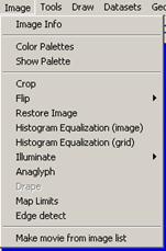 Provides info about the current image. If the image is derived
from a GMT grid the output is the one issued from grdinfo. If it
is a common format image, the info includes only the number of
rows and columns of the image and if it is a true color image
(rgb) or an indexed image. If the image was read by the GDAL
interface, a more extended info is provided (uses the output of
gdalinfo). In that case an even more complete report (for
example if the image/grid has projection information) may be
found on the Mirone “tmp” directory. Search for a file with the
same name as your image and with a .info extension.
Provides info about the current image. If the image is derived
from a GMT grid the output is the one issued from grdinfo. If it
is a common format image, the info includes only the number of
rows and columns of the image and if it is a true color image
(rgb) or an indexed image. If the image was read by the GDAL
interface, a more extended info is provided (uses the output of
gdalinfo). In that case an even more complete report (for
example if the image/grid has projection information) may be
found on the Mirone “tmp” directory. Search for a file with the
same name as your image and with a .info extension.
·
Color
Palettes - Opens a window tool from where you can select
 between more than 100 color tables. Every selection takes place
immediately. Every time that a new color schema is selected the
base image is automatically updated. Furthermore, all palettes
may be changed by a double click over the color bar. That
inserts color markers. Drag these markers to modify the color
map. A second double click deletes the marker. 'The Min Z
and Max Z fields may be used to impose a fixed color map
between those values. External GMT color palettes may also be
imported or exported via the File menu. Note: If you have
previously drawn contours into your image, you can easily fit
the colors with the contours.
between more than 100 color tables. Every selection takes place
immediately. Every time that a new color schema is selected the
base image is automatically updated. Furthermore, all palettes
may be changed by a double click over the color bar. That
inserts color markers. Drag these markers to modify the color
map. A second double click deletes the marker. 'The Min Z
and Max Z fields may be used to impose a fixed color map
between those values. External GMT color palettes may also be
imported or exported via the File menu. Note: If you have
previously drawn contours into your image, you can easily fit
the colors with the contours.
· Show Palette - Shows the color palette of the currently displayed image (this a rather pedestrian tool)
· Crop - Crops an image to a specified rectangle. Press the left mouse button and drag to define the crop rectangle. Finish by pressing the left mouse button again. Note, this is crude and little controlled way of doing a cropping operation. The best way is to draw a rectangle on the image. Calmly decide on its size and position and than inquire its properties (by a right-click on the rectangle borders) for “Crop Image”.
· Flip - Flips the image UP-Down or Left-Right. Note: coordinated (georeferenced) images are displayed with origin at lower left corner and plain images with origin in upper left corner. Some operations like referencing or draping require knowing where to flip or not one image with respect to the other. Although I try to keep trace of this, sometimes I get caught in an unexpected case, and the result is upside-down. Use this option if that happens.
· Restore image – Restores the original image. Use this if you have been playing around with the color palette tool or histogram equalization and want to start over.
· Histogram Equalization (image) - Enhances the contrast of images by transforming the values in an intensity image, or the values in the color map of an indexed image, so that the histogram of the output image approximately matches a flat histogram. This operation works pretty well for black and white images but give somewhat idiot results for color images. The reason relies on the fact that for color images each color band is independently equalized and then a color image is rebuilt. I know that's not the way the thing should be done, but the correct operation (which is followed in Region-Of-Interest) is very slow and memory consuming. When an image is equalized, the original image is saved in memory and selecting this operation again restores that original image. This can be used for undoing other image operations (like illuminations).
· Histogram Equalization (grid) - Follows the same strategy as in the grd2cpt GMT program. Here, I calculate a new color palette based on the grid’s cumulative distribution function (CDF). One basic difference regarding the image histogram equalization option is that it operates directly on the grid values, and not on the derived image. That means NaNs are ignored and won't affect the final result (contrary to the image version). On the other hand, the end result is often not so nice - possibly because I'm not doing it correctly.
·
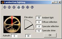 Illuminate
- Provides alternate schemas to do image illumination. A window
tool allows selection of inclination and azimuth of the light
source. Among the available options, the False Color lets
you illuminate a GMT grid along three different directions and
compose the final image with each illuminated direction in the
three color channels (R, G and B). This is useful for enhancing
structures perpendicular to each of the selected direction.
Illuminate
- Provides alternate schemas to do image illumination. A window
tool allows selection of inclination and azimuth of the light
source. Among the available options, the False Color lets
you illuminate a GMT grid along three different directions and
compose the final image with each illuminated direction in the
three color channels (R, G and B). This is useful for enhancing
structures perpendicular to each of the selected direction.
· Anaglyph - Produces an image that, when seen with red-blue glasses, gives a 3D perception view.
· Drape - For having access to this option you need to have two Mirone windows opened. Then, the image of the second opened window can be draped on the first one. If the fist image results from a grid you can still elaborate (complicate) more by applying an illumination. That illumination will change the Hue (from the HSV model) of the first image. Finally, this image can be saved with the Save As 3 GMT grids (R,G,B) option. Imagine that the first image was obtained from loading a GMT grid DTM model and the second represents a satellite image (or aerial photograph) of the SAME region. At the end you will have the GMT grid and the draping image split into three RGB grids. You can then use GMT4.0 to drape the three grids version of your photo onto the DTM. Notice that the image quality will be degraded to fit the DTM resolution. This option is also useful if you want to drape an image on a DTM before computing a Fledermaus object. A good example is to drape a backscatter image (preferable pos-processed with the ROI options) over a multi-beam bathymetry.
· Map Limits - When you have a non referenced image (a scanned image for example), use this to set the image coordinate limits. A better way of doing this is provided by the option Register Image available by right mouse clicking onto rectangle elements.
· Edge detect – Run an edge detection algorithm (the MATLAB canny algorithm) over the displayed image and plots the result as polylines that may be saved as ascii files. This is more than the traditional edge detecting operations do. Note that the edge detecting is carried out over the image after it has been converted to a gray image and not on the grid that it derives from. So instead of letting the code do the conversion to a gray scale you better do it yourself and eventually shade that image. This way you have much better control on what is going to be edge detected.
· Make movie from image list – Provide an ascii file with a list of images files (one per line) and get back an AVI animation made up of those images. The images may be in any of the images recognized formats, but they obviously must all be of the exact same size.
Tools menu
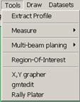 ·
Extract
Profile - Left clicks will plot a polyline, a right click
remove the last entered point, double click to stop. As result a
new window will pop up with an x,y plot containing
the profile extracted from the grid along the drawn track. This
corresponds to an interactive version of the grdtrack GMT
program. The profile thus obtained can be saved to disk. Note
that the x,y profile coordinates are obtained from linear
interpolation and by consequence on geographic grids they may
differ reasonably from the great circle arcs that reflect the
shortest distance on a sphere between the end points. Note, this
is crude and poorly controlled way of doing the profiling
operation. The best way is to draw a line or polyline on the
image. Calmly decide on its position and than inquire its
properties (by a right-click on the rectangle borders) for
“Extract Profile”.
·
Extract
Profile - Left clicks will plot a polyline, a right click
remove the last entered point, double click to stop. As result a
new window will pop up with an x,y plot containing
the profile extracted from the grid along the drawn track. This
corresponds to an interactive version of the grdtrack GMT
program. The profile thus obtained can be saved to disk. Note
that the x,y profile coordinates are obtained from linear
interpolation and by consequence on geographic grids they may
differ reasonably from the great circle arcs that reflect the
shortest distance on a sphere between the end points. Note, this
is crude and poorly controlled way of doing the profiling
operation. The best way is to draw a line or polyline on the
image. Calmly decide on its position and than inquire its
properties (by a right-click on the rectangle borders) for
“Extract Profile”.
· Measure - This is a measure tool that allows measuring distances (in units selected in Preferences), azimuths in degrees (cw from north) and area (in km2). Start by a left clicking and proceed with as many left clicks as you want. A double-left click adds the last point and shows up the results. Right clicks remove the previously entered point.
· Multi-beam planning - This tool is meant to help the planning of multi-beam surveys. Various systems have different swath widths coverage that depends on the number of beams of the particular system and the water depth. For simplicity the bottom coverage can be assumed to be a relation of the water depth. Hence, a "swath-width / water depth ratio" of 2 means that on a 4 km water column the swath will have a width of 8 km. The facilities provided are:
a) Start a new track. In this mode left-clicks add new points; right-click or pressing the delete or back space remove previous points. Pressing RETURN, ENTER or middle button click ends the track and asks for a file name to save the track on disk.
b) Imports a track from a (x,y) file on disk.
c) Edit a track. In this mode the first left-click selects the track to be edited. The second selects the closest vertex that can now be moved and place into a new position by another left-click. However, while in the edit mode, pressing the "r", DELETE or BACKSPACE keys will remove the vertex; pressing "i" will insert a new vertex; pressing the "b" key will break the track in two. RETURN or left-click stops the edit mode.
d) Delete a track. Use left-click to select the track and right-click to confirm.
e) Save the track on disk. Use left-click to select the track and right-click to confirm.
f) Compute the track length in Nautical Miles. Computations are made using great circle distances and spherical Earth approximation.
· Region-Of-Interest - Use left mouse clicks to draw a closed polygon. A double left click ends the polygon drawing. Then you can select from a list of image processing operations that will be applied only inside the ROI polygon. Those operations work pretty well for grey images but regarding color images they may be very slow. That happens because the whole color image has to be transformed into an intensity space (YIQ in current case) and back to RGB, and those are slow operations and VERY memory demanding as far as Matlab is respected. So, even if you start with an indexed image you'll end up with a true color (RGB) image.
· X,Y grapher – Calls the X,Y tool in a empty mode. Use this if you want to load a x,y file.
· gmtedit – gmtedit was an old GMT program from the time of version 2 that used to run only in Sun stations with the openview OS. Most of you don’t even know what I’m talking about. However, it was a very useful program to view and edit the .gmt files created and manipulated by the GMT supplements mgg. If you still don’t know what I’m referring to probably the best is to jump ahead. Well because I needed it I decided to resuscitate gmtedit. I don’t show a picture of it here because it occupies the whole screen. Its use is very easy. Load a .gmt file and click on the points that you decide are outliers. They will turn red (bad points). Another click will make them green (good points) again. The first rectangle icon allows doing this selection by area. The second only applies to the magnetic channel and permits to move the points by dragging the rectangle. At the end save the edited file. Red marked points will be replaced by the no-data-value.
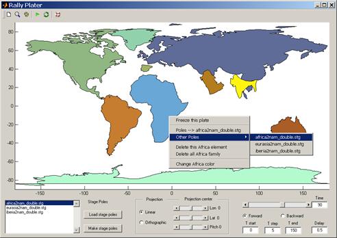
· Rally Plater – This tool lays somewhere between a Plate reconstruction demo and something that can be used to do real work. There are some dedicated softwares available on the web that do plate reconstructions but this one has a big advantage. It is ready to work upon start, and is very easy to use. There is no need to explain what the buttons do. They self explain with their tooltips. To access other fundamental options right-click over the "plates". New menus popup and is there that the user controls how the plates move. By default the program associates a “movement history” to three plates: Iberia, Eurasia and Africa. The movement is defined by the poles that show up in the window’s lower left corner. In addition to the default files, the user can load its own data. There are two types of data: the poles files, which control how the plates move; and the plates files.The poles used in this program are stage poles (not finite rotation poles). They have a particular format described in detail in the rotconverter GMT program, but the example files can be found at them at the "continents" directory of Mirone’s installation. To create new stage poles files from finite rotations poles hit the "Make stage poles" and follow instructions there. The plates files are simple ascii files with two columns: longitude and latitude (in that exact order). Now, those files may be multisegments, with the character ">" serving as the separator. The individual segments may be closed (equal first and last point). If they are closed, the contour is filled, otherwise they are drawn as lines. Very important: The first line in file must be of the form ''# Name'' (without the quotes), where Name is the plate’s name. This is the mechanism that the program uses to know how to associate a plate and its companion lines with a stage pole. We can see the default plates name when right-clicking over it, so if we want to add it another element (e.g. the 3000 m bathymetric) we must give in that file the exact same name as the plate we want it to join.
Draw menu
NOTE: All graphic elements drawn with the options in this menu are given a lot of properties that include changing the line style, color, thickness, editing, deleting and so on. For accessing to these properties just right click on the selected element and choose what you want to do.
·
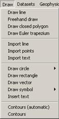 Draw
line - Use left mouse clicks to
draw the line (in fact a polyline) and stop with a double left
click. You can use these line to extract a profile from the grid
(if it is the case) where it was drawn.
Draw
line - Use left mouse clicks to
draw the line (in fact a polyline) and stop with a double left
click. You can use these line to extract a profile from the grid
(if it is the case) where it was drawn.
· Freehand draw – Draws a line that follows the mouse movement. Start with a left-click and stop with a double-click. While drawing hit the “c” key to close the line.
· Draw closed polygon – Do what it says. End with a double-click.
· Draw Euler trapezium – This a special tool to fast compute an Euler pole using the so called Bonin method. It works in the following way. You draw a trapezium (in much the same way as you draw a closed polygon). Then right click on it and select “Compute Euler Pole”, the result will appear either on the ML command window or in the dos window if you are running the stand-alone version. Now what it does. First and second points define side A, third and fourth the side B. The side A is rotated to fit over side B. This involves two separate rotations. The first rotation brings points 1 and 4 together. A second rotation is than performed, about the now coinciding points 1 and 4, by the angle defined by the first line segment (the one that originally made up by points 1 and 2) AFTER the first rotation and the second line segment (original points 3 and 4). The result is the combination of the two rotations. Though it is a crude method, it sometimes gives very good results. If you don’t know what I’m talking about, just forget this option. If, on the other hand you do, you can thank me.
· Import line - Prompts for a file name of an x,y ascii file that will be drawn as a line on the current figure. That line will be given the same properties as the natively drawn lines.
· Import points - Prompts for a file name of an x,y ascii file that will be drawn as individual points on the current figure. Points will be given the same properties as the natively inserted symbols.
· Import text – Import text from an ascii file. That file must have the x,y coordinates in the first two columns, followed by the text.
· Draw closed polygon - It works much like in Region-Of-Interest except that (1): you are not prompted to do any other operation. However, the same ROI operations are available by right clicking on the ROI polygon. (2): You can use the polygon to do an alternative "Crop Grid". The croping rectangle is defined by the x,y polygon min and max limits, and the grid nodes outside the polygon are set to a constant value prompted to user.
· Draw Euler trapezium –
· Draw circle - Draw circle lets you draw small circles in geographic coordinates (or plain circles with cartesian coordinates). The three sub-options available are Geographical Circle where the first left click defines the circle center and the second a point in the perimeter. Meanwhile, moving the mouse draws the circle on the fly. The second sub-option Circle about an Euler pole lets you select the circle's center from a relative (or absolute) Euler pole, selectable from the popup menus in the window that will be opened. Once you made your pole choice, the center is already defined and you only have to give another left click to select a point on the perimeter. Now, if you want to change the circle’s radius or move it double click on the circle. The center (if visible on the figure) is shown by a red point. Click and drag to move the circle. The radius can be changed by click and dragging the red circle on the perimeter. These and other settings may be also done in the parameter window that has meanwhile shown up. Double clicking again removes the circle’s editing properties. If the circle is of the Circle about an Euler pole type, right clicking lets you choose to calculate the Euler velocity on the point where the red circle is displayed. The third sub-option lets you draw a Great circle arc.
· Draw rectangle - Works pretty much in the same way as the circle’s case, except that the given properties are different. You can now crop images and/or grids, change/move the rectangle and so on. Relatively hidden in these properties is the possibility of using the rectangle coordinates to register an image. This is more correct and gives more freedom to the user than the Map Limits option. The rectangle corner coordinates are used to compute an affine transformation that registers the image to the rectangle's coordinate system. To compute an affine transformation we need at least 3 points. With the rectangle we have 4, which is ok but imposes the unnecessary (to the affine transformation) restriction that the points lay on a rectangle. In fact, if you edit and change the rectangle to another shape, the registration option will no longer be available. I intend to change that, but it will require writing a new graphical tool specific for the purpose. From the rectangle properties you can also select the Transplant Image here. This is a non-finished tool that allows selecting a second image that will be inserted inside the area enclosed by the rectangle. In its current state, the second image is always reinterpolated to fit the space (in terms of rows and columns) inside the rectangle. The crop tools options provide useful options that apply only to the grid elements contained in the rectangle. I wrote the spline smooth, median filter and fill gaps having in mind post processing of swath bathymetry grids. Mainly to disguise the region of overlapping swaths. While this works pretty well (you may even work on shaded illuminated images) it has one drawback. It may leave a too clear suture zone between the processed and non-processed zones. This option has a experimental undo.
· Draw vector - Draws a vector by the same clicking sequence as above. However, this cannot be edited. Only deleted.
· Insert symbol - Filled circles, squares, triangles and stars are plotted by a left click. Right clicks on these elements lets you change size, fill and border color, select other symbols ...
· Insert text - Left click for the point of text insertion and then write whatever you want. Left click (do not hit ENTER unless you want to change line) outside the text box to end. If you have previous line elements you will notice that they vanished when you started ton write your text. Don’t worry, it’s just an innocuous Matlab BUG (it has many). To get back all your stuff click on the refresh button (the one with two curved arrows) of the Mirone button collection. Text may be edited and moved or change the font, size, color by accessing its properties (again, right click on it).
· Contours (automatic) - For grids, this automatically calculates and draws a set of contour lines.
· Contours - Raise an option window where you can select which contours to draw.
Datasets menu
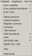 ·
Draw
coastline, Draw political boundaries, Draw rivers
- Use the netCDF GMT database. Depending on what you installed
in GMT so you will access to the crude, low, intermediate or
full resolution files. Needless to say that drawing coastlines
will only work with geographic registered images.
·
Draw
coastline, Draw political boundaries, Draw rivers
- Use the netCDF GMT database. Depending on what you installed
in GMT so you will access to the crude, low, intermediate or
full resolution files. Needless to say that drawing coastlines
will only work with geographic registered images.
· Earthquakes - Select earthquakes with magnitudes >= 5 for the period 1990-2003. Seismicity from the NEIC web site.
· Hotspot locations - For those of you that are Hotspotist this option plots the (B. Steinberger, JGR, v105, p11127--11152, 2000) Hotspot locations list. Right clicking lets you ask for the ghost name.
· Magnetic isochrons - Plots the Muller et. all. Digital Isochrons of the World's Ocean Floor. Right clicking on individual isochrons provides a short info about it.
· Volcanoes - Plots the Smithsonian volcanic activity list. Again, right clicking on an event gives access to a short description of it.
· Tide Stations – This will plot the tidal stations of the t_xtide.mat file that resides in the “data” directory. Once the tidal stations are plotted in your base figure, right clicking gives access to either the station info (name, location, nº of harmonic coefficients, etc) or to the “Plot Tides” option. This will open a new window showing the tides for a period of two days more or less centered in the current date. This window mimics the original WXtide program but does not offer all the possibilities of the original program (no tide calendar, etc). The t_xtide.mat file was converted from the harmonics file contained in WXtide (version 2.6) using the t_xtide.m code of the “tides” toolbox (Pawlowicz et al., Computers and Geosciences, 28 (2002), 929-937). In fact most of the computing code of this tool was extracted from t_xtide. Users that interested on knowing more about the harmonics used in this program are directed to the WXtide (just search for it on the web) help files. You will also find there instructions on how to compute new harmonics files (if you have the data for doing it). WXtide comes with more harmonics files. In case that you are interested to use one of them instead of the one provided here, use “Harmonics to mat file” option to generate a new t_xtide.mat and replace it by the original one.
· Plate Boundaries - Draws the P. Bird (element.ess.ucla.edu) plate boundary list. Different boundary types are plotted with different colors. Right clicking on a boundary gives access to the boundary type, neighbouring plates and velocity across that boundary. I slightly changed the original file for the Açores Triple Junction region.
· Cities - Selects the Major cities or Other cities to plot city places and names. I recovered these files from the iGMT distribution.
· ODP/DSDP sites - Plots either the ODP or the DSDP (or both) sites. Right clicking on a site lets you have access to minimalist site information.
· Magnetic Bar Code - Opens a window with the Cand & Kent (1995) Magnetic inversion time scale.
· Atlas – This tool is at a rudimentary stage but it works ok. The GMT coastlines are built in such a way that they don’t allow plotting individual countries. I built up a new (simple) database made by countries defined individually and wrote a C program to read it. You may select a country or a whole continent. If a base Mirone window exists than the country as a patch is added to it, otherwise a new area is created to receive that country. Now countries may be attributed properties accessible by a right-click. However, I found out another very unpleasant MATLAB feature. Attributing properties using uicontexts (that’s the technical description) is VERY VERY memory consuming. To give you an idea the whole world at the maximum resolution swallowed me more than 500 Mb of RAM. Meanwhile I reduced the number of uicontexts but it still consumes about 200 Mb for the whole world (can we believe that?). And more, killing the figure may take more than 30 seconds (these ML guys…). So, think twice before checking the “Provide controls to polygons” option if you are loading many countries (but for a small number you don’t notice this). Bonus, the “Write GMT script” option knows how to deal with these data a will make a nice GMT ps figure.
· External db – This a somewhat poor name for what it does. If you have multisegments (in the GMT sense) ascii files you may use the separator line to add information to it. Example, “> Anomaly 5 Eurasia/NAm”. Here the “>” is used to indicate a new segment and the text that follows is the line tag. When imported that line it will be named accordingly to its tag. A right-click on the line will show the tag info. This is very useful if you import many lines and don’t know anymore which is which in a crowded Mirone window.
Geophysics menu
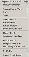 ·
Elastic
deformation - Here you can either import a line (or
polyline) or draw it over your image grid. That line is than
interpreted as a surface trace of a fault. Right clicking on the
line will show (among others) two options to call new windows
where you will specify the fault parameters (width, depth, dip)
as well as the movement you will simulate. The two available
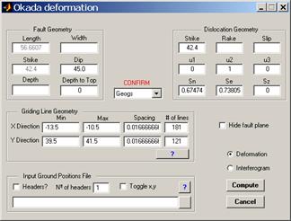
options are called Okada and Mansinha.
The Okada window is more general and here you can:
model co-seismic displacement - that can be compared with GPS
measuring - for an initial condition of the far field tsunami
modeling (see bellow) or to compute synthetic interferograms.
The Okada window provides short help in the form of tooltips
when the mouse rests a bit over individual entry boxes. For a
complete reference you must read the
·
Elastic
deformation - Here you can either import a line (or
polyline) or draw it over your image grid. That line is than
interpreted as a surface trace of a fault. Right clicking on the
line will show (among others) two options to call new windows
where you will specify the fault parameters (width, depth, dip)
as well as the movement you will simulate. The two available
options are called Okada and Mansinha.
The Okada window is more general and here you can:
model co-seismic displacement - that can be compared with GPS
measuring - for an initial condition of the far field tsunami
modeling (see bellow) or to compute synthetic interferograms.
The Okada window provides short help in the form of tooltips
when the mouse rests a bit over individual entry boxes. For a
complete reference you must read the
RNGCHN paper (Feigl and Dupre 1999; Computers and Geosciences, 25 (6) pp. 695-704). The paper and the source code used to be available on authors ftp site but it seams to have vanished.
The Mansinha option computes only the vertical component of the deformation produced by an earthquake. The two codes should produce equal results (and they very closely do). On both Okada and Mansinha, a clever guess is made about the type of the grid coordinates. Accepted types are geographical, meters and kilometers. While the guessing works well most of times it may also fail, so please pay attention to the guessed type and corrected if it is not correct. When working with geographical coordinates all distances are computed by previously projecting the geographical coordinates to Transverse Mercator with origin in fault's first point. Next figure shows an example of Okada use. Not shown in that figure is the one more of the Mirone’s fine details. The horizontal projection of the fault(s) plane(s) are displayed on the main window.
· Tsunami Travel Time - Computes the tsunami travel time according to equation v = sqrt(gH), where g is the gravity acceleration and H is the water column depth. To use it, first plot the source location (note: you can give it an exact location), than right click on the source symbol and select Compute. That's all, depending on your grid size the result will appear immediately or wait a bit.
Alternatively you can load a file with x y time records (one per line) using the Import maregraphs and time option. Here the x y time represent, respectively, the coordinates and time of arrival at the tide gauge stations. The Compute will compute the tsunami source location using a least squares estimation of the backward ray-tracing time. Pay particular attention that none of your tide gauges is on land (that is, its depth must always be negative), otherwise the result is NaNs (NaN = Not A Number) and the shown image is all white.
·
 Swan
- Use the Mader's SWAN code to model tsunami propagation. To use
this program you need to have two grids that are EXACTLY
compatible. This means they must cover the same region and have
the same number of rows/columns. One of the grids represents the
bathymetry (z positive up) in meters and other contains the
initial deformation as produced by the Okada deformation
module. The next thing you need is a parameter file. In the
"data" directory of the root Mirone installation you will find a
file named swan.par. Use this as an example for your case. I
don't know the purpose of most of the parameters, only of those
who seams to be important. The swan.par has short comments in
front of each parameter.
Swan
- Use the Mader's SWAN code to model tsunami propagation. To use
this program you need to have two grids that are EXACTLY
compatible. This means they must cover the same region and have
the same number of rows/columns. One of the grids represents the
bathymetry (z positive up) in meters and other contains the
initial deformation as produced by the Okada deformation
module. The next thing you need is a parameter file. In the
"data" directory of the root Mirone installation you will find a
file named swan.par. Use this as an example for your case. I
don't know the purpose of most of the parameters, only of those
who seams to be important. The swan.par has short comments in
front of each parameter.
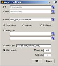
Now that you are ready to do the simulation you have to choose between computing the simulation on specific points - called maregraphs here - or on the whole grid region. If you want the first option, than you either plot those stations graphically (using the Plot Stations option) or import a x,y file with the maregraphs location. This later option is also available in the swan_options window. If you want to compute the simulation in the whole region, than proceed with the Compute option. In the swan_options window you will finally select what to do. The Bat and Source edit boxes must contain either the name of your grids or a gray line with the In memory array string, which appears when the Swan module was called from a Mirone window in which a valid grid was previously loaded. In the Params edit box you load the swan.par parameter file mentioned above. If you already plotted stations in the bathymetry window grid the Maregraphs section will be automatically set, otherwise check the check box and give the necessary file names to compute the maregraphs (in case you want to do it - not mandatory). Maregraphs are nothing but a record of the water height vs time at a certain location(s). The Output grids check box tells the program that you want to write grids on disk containing the water height at particular time intervals of the simulation cycle. For example if in the swan.par dt = 1 and cumint = 30 that means the simulation is computed at increments of one second and grids (as well as maregraphs if that option was selected) are written at every 30 seconds of the simulation. Grids are automatically named after the name template provided in the edit box appended with the cycle number. As an alternative to writing grids on disk, you can compute an AVI movie. In Nº of cycles you select for how many cycles will the simulation be run. Again, using the same example of dt = 1 the default value of 1010 means the simulation will extend for 1010 seconds.
I left behind on purpose the Plot stations on grid borders Swan option. This option's purpose is meant only for using in the Tsun2 module (see bellow).
· Tsun2 - Use the Imamuras's tsun2 code to model a tsunami inundation. Although the SWAN code has a parameter called flooding I don't know how to use it. Instead I use the tsun2 code to compute the coastal flooding simulations. In order to that these simulations are realistic, they have to be run over small areas described by very detailed DTMs that include both topography as well as bathymetry data. The so called far field codes are not appropriate to model coastal inundations and the shallow water models (like tsun2) use such a small grid spacing that for the sake of running time is jus not practicable to make them run since the earthquake epicenter until the coast. The strategy is than to use a far field model to compute the tsunami propagation using a coarse grid spacing (typically about 1 km) until near shore and than use this simulation to feed a shallow water code.
The tsun2 code thus runs on a very fine grid mesh - with grid spacing typically not superior to 50 meters - and must be feed at every grid node of one or two of its grids borders. The feeding procedure consists in providing a maregraph record for all grid nodes of the border(s) at which the external wave arrives at the finer grid. However, as mentioned above, this is impracticable because it would imply running an external feeding code (Swan in this case) at the same (very fine) grid spacing as the fine grid. The solution adopted was than to use finer grids that have grid node spacing that are sub-multiples of the coarse grid. For example, dx = 50 m equals 1 km / 20. That way we insure that every 20-th +1 finer grid node will coincide with one node of the coarser grid. To complicate a bit more (but safer against misalignments) it is desirable that the origin coordinates of the finer grid coincide with those of one node of the coarser grid. With these conditions meat, feeding all grid nodes of the finer grid is simply accomplishing by linear interpolation of the water height using data at nodes actually feed by the far field code (one every 21 in the example above). It is a user task to construct such a pair of coarse/fine grids using a cartesian coordinate system (e.g. UTM).
It is now that the Plot satations on grid borders option in Swan comes handy. By selecting this option the finer grid is loaded and all its grid nodes around the four borders will be plotted on the figure derived from the coarse grid (if you doubt it, zoom in until you are convinced). Here a previous knowledge of the direction from which the tsunami arrives is required. Remove the borders at which the tsunami cannot arrive (that is, without crossing the smaller area). That will leave you with at most two frontiers. Now run Swan and save the maregraph file. That file is the one you need to feed in the Tsun2 module, but before you can run it there is still one last step. Select Write params file in Tsun2 entry and save a new parameter file (this time for Tsun2). This file contains indexes information used to translate the maregraph file created by Swan into coordinates of the finer grid used in Tsun2. Selecting Compute popup an option window very similar to the Swan’s options window. In fact it contains only one extra option which is Jump initial. Leave the mouse pointer on it and the tooltip should be self-explanatory.
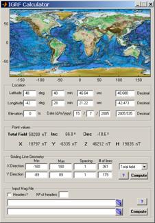
· IGRF calculator - Calls the IGRF calculator tool where you can compute the value of the total magnetic field (or its components) either on a given point, generate a grid of regularly spaced magnetic quantities or read a file with at least lat, long positions. When used to import a file, a new window pops up where you select which data column means what. You have here the possibility to choose to compute the magnetic anomaly (measured total field - IGRF magnitude). Computing magnetic anomaly requires knowing the date of measuring. The reading file function has the ability to decode many date formats (that's why it may be a bit slow to read large files) including text formats. Hit the "?" button for help in text date formats. The IGRF model used is the 10th generation IGRF as agreed in December 2004 by IAGA Working Group V-MOD. It is valid 1900.0 to 2010.0 inclusive. Values for dates from 1945.0 to 2000.0 inclusive are definitive, otherwise they are non-definitive.
·
 Parker
direct, Parker inversion and Reduction to the Pole - are
standard procedures used in magnetic field modeling. It is out
of scope of this document to explain the principles behind those
methods. Either you know them and than the use of these modules
should be pretty obvious or you don't. If you do not know and
want to learn, I suggest that you start by reading the
Blakely textbook. The credit to these modules goes mainly to
Maurice Tivey for I used functions from his magnetic toolbox as
backbones to write them.
Parker
direct, Parker inversion and Reduction to the Pole - are
standard procedures used in magnetic field modeling. It is out
of scope of this document to explain the principles behind those
methods. Either you know them and than the use of these modules
should be pretty obvious or you don't. If you do not know and
want to learn, I suggest that you start by reading the
Blakely textbook. The credit to these modules goes mainly to
Maurice Tivey for I used functions from his magnetic toolbox as
backbones to write them.
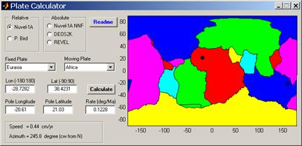
· Plate Calculator - Opens a window tool from where you can calculate plate velocities according to the available models (e.g. NUVEL1A, REVEL, DEOS2K). It has a help of its own but its use is as simple as clicking on the image.
·
Geographic calculator
-  This tool is an interface to both mapproject and grdproject.
It uses a mex version of these programs and its use should be so
trivial that no help is needed (well, for users that know what
they are doing). GMT4
introduced datum conversions in mapproject
(but not in grdproject) and shifts that allow conversion between
the
plethoras of projection systems used all over the world. In
Mirone I coded only the Portuguese systems. I hope in this way
to contribute to end the "state top secrete" issue that seams to
exist around this matter (if you are Portuguese and need to do
coordinate conversions from/to national systems I'm sure you
understand what I mean). For other countries, I still need to
invent a way to allow them to define their projection systems.
Overall, this tool frees GMT users from the need to provide a
correct -R (potentially particular hard to know in
advance in inverse transformations), and prevented many users
(me included) to be able to use grdproject.
This tool is an interface to both mapproject and grdproject.
It uses a mex version of these programs and its use should be so
trivial that no help is needed (well, for users that know what
they are doing). GMT4
introduced datum conversions in mapproject
(but not in grdproject) and shifts that allow conversion between
the
plethoras of projection systems used all over the world. In
Mirone I coded only the Portuguese systems. I hope in this way
to contribute to end the "state top secrete" issue that seams to
exist around this matter (if you are Portuguese and need to do
coordinate conversions from/to national systems I'm sure you
understand what I mean). For other countries, I still need to
invent a way to allow them to define their projection systems.
Overall, this tool frees GMT users from the need to provide a
correct -R (potentially particular hard to know in
advance in inverse transformations), and prevented many users
(me included) to be able to use grdproject.
·
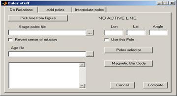 Euler
rotations - Rotating magnetic
isochrones or creating flow lines is very easily accomplished
using this tool. Any line element, either drawn or imported from
an ascii file, or point symbol may be rotated using either a
stage pole file like the ones described in the Rally Plater
tool or using a finite rotation pole. For selecting a line or
point do a single left-click on it. The selected element will
than show red stars in its vertices. Next, right-click on any
free zone of the image to confirm the selection (the red stars
will disappear). When used to do rotations with stage poles it
is also necessary to provide an age file which determines the
ages at which the rotation is computed. For each entry of that
age file (displayed in the window’s listbox) a new rotated line
is plotted in Mirone main window. The “Magnetic Bar Code” button
provides an easy way to select an age sequence using the
geomagnetic polarity scale as reference. For using it one has to
double-click over the period bars. A marker, as well as new
window with its age will show up. Insert as many age
markers as wanted and drag them to fine adjust the wanted time.
Euler
rotations - Rotating magnetic
isochrones or creating flow lines is very easily accomplished
using this tool. Any line element, either drawn or imported from
an ascii file, or point symbol may be rotated using either a
stage pole file like the ones described in the Rally Plater
tool or using a finite rotation pole. For selecting a line or
point do a single left-click on it. The selected element will
than show red stars in its vertices. Next, right-click on any
free zone of the image to confirm the selection (the red stars
will disappear). When used to do rotations with stage poles it
is also necessary to provide an age file which determines the
ages at which the rotation is computed. For each entry of that
age file (displayed in the window’s listbox) a new rotated line
is plotted in Mirone main window. The “Magnetic Bar Code” button
provides an easy way to select an age sequence using the
geomagnetic polarity scale as reference. For using it one has to
double-click over the period bars. A marker, as well as new
window with its age will show up. Insert as many age
markers as wanted and drag them to fine adjust the wanted time.
If a single point was selected (using the “Pick line from figure” button) instead of a line/polyline, than a single flow line is plotted. In the “Add poles” tab the user may compute the pole that results from a combination of two finite rotations.
With this tool you can also add or interpolate poles. Pay attention to the tooltips.
·
Compute
Euler pole - 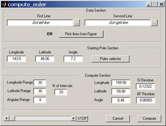 Users that want to compute their own Euler
poles can do it with this tool. For using it all is needed are
two lines in the main window, which will be mouse selected after
hitting the “Pick lines from figure” button, and an initial
estimate of the Euler pole. For selecting the lines follow the
same procedure as described above for Euler rotations.
That is: left-click to select and right-click to accept – once
for each line. The results of the searching algorithm are
graphically displayed every time a better fit pole is found. If
at the end of the process the user is not fully satisfied with
the result, all that he needs is to restart again using this
time a better initial guess of the starting pole.
Users that want to compute their own Euler
poles can do it with this tool. For using it all is needed are
two lines in the main window, which will be mouse selected after
hitting the “Pick lines from figure” button, and an initial
estimate of the Euler pole. For selecting the lines follow the
same procedure as described above for Euler rotations.
That is: left-click to select and right-click to accept – once
for each line. The results of the searching algorithm are
graphically displayed every time a better fit pole is found. If
at the end of the process the user is not fully satisfied with
the result, all that he needs is to restart again using this
time a better initial guess of the starting pole.

· Manual adjust Euler pole – If you want to do either a free rotation of a line or try to fine tuning one pole, you can use this tool. Again, you select a line, enter the pole parameters and move the sliders. The line is rotated accordingly. Try it and find out how is far from trivial to fit two lines.
·
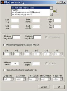 Seismicity and focal
mechanisms – The figures above
show the two interfaces to plot either epicenters locations or
Seismicity and focal
mechanisms – The figures above
show the two interfaces to plot either epicenters locations or
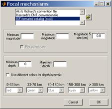 draw focal mechanisms (the seismologist’s beach balls). To plot seismicity use either an ascii file with data in lines organized
as: lon, lat, depth, magnitude, year, month, day, [hour, minute,
second]. As an alternative one may use a ISF formatted catalog
(like the ones we can get from
www.isc.ac.uk). Reading the ISF format is done with a mex
file. A “Posit file” reads the format used by PMEL to divulgate
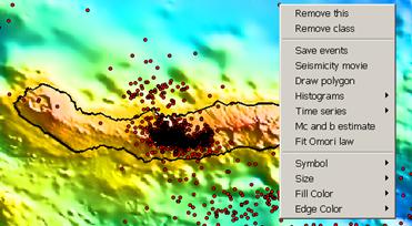
the hydrophone detected seismicity. Once you have loaded a
seismicity file, there are many operations available trough a
right-click. Namely, play a seismic movie (a separate window
controls the “movie” parameters), display several types of
histograms and fit a Modified Omori Law. This later as
well as the Mc and b value estimate was taken from parts of code
of the Zmap toolbox. A finer refinement is achieved when we
select to “Draw a polygon” around an interest area. Then the
same options are available but will apply only to the data
contained inside the polygon. It contains also a tool to detect
swarms. That is a very basic tool that uses a home made
criterion of space and time distances to detect the events
connectivity.
draw focal mechanisms (the seismologist’s beach balls). To plot seismicity use either an ascii file with data in lines organized
as: lon, lat, depth, magnitude, year, month, day, [hour, minute,
second]. As an alternative one may use a ISF formatted catalog
(like the ones we can get from
www.isc.ac.uk). Reading the ISF format is done with a mex
file. A “Posit file” reads the format used by PMEL to divulgate
the hydrophone detected seismicity. Once you have loaded a
seismicity file, there are many operations available trough a
right-click. Namely, play a seismic movie (a separate window
controls the “movie” parameters), display several types of
histograms and fit a Modified Omori Law. This later as
well as the Mc and b value estimate was taken from parts of code
of the Zmap toolbox. A finer refinement is achieved when we
select to “Draw a polygon” around an interest area. Then the
same options are available but will apply only to the data
contained inside the polygon. It contains also a tool to detect
swarms. That is a very basic tool that uses a home made
criterion of space and time distances to detect the events
connectivity.
To plot focal mechanisms one can use the formats shown in the list. In the Aki & Richard’s convention the data is ordered as: lon lat depth strike dip rake (in degrees) magnitude. Optionally add two more columns with the lon and lat at which to place the beach ball. The Harvard’s CMT convention uses: lon lat depth str1 dip1 rake1 str2 dip2 rake2 mantissa and exponent (of moment in N-m). Again, optionally add two more columns with the lon and lat at which to place the beach ball. WARNING, contrary to psmeca, the moment magnitude uses N-m (and not Dyn-cm). Also, it is not yet possible here to have a last string column containing the event label. However, the ISF formatted files uses the event date to build up an event label.
A big advantage of using the focal mechanism tool over using psmeca is that the user may easily displace the beach balls using the mouse. This is particularly useful when we have a lot of events on top of each others. Also, the Write GMT scrip tool is able to detect beach balls and to make the appropriate calls to psmeca that reproduce the graphical display.
· Import *.gmt file(s) – A .gmt file is handy format to store the Gravity, Magnetics, Topograpy data contained in the mgd77 exchange format file provided by NGDC. Read the GMT mgg supplement manuals to learn more about the format and how to create .gmt files. These options let you import either one gmt file or a list of files. The list of files is a simple ascii file with the full path of each gmt file, one per line. Once read, the files appear as tracks in the figure. Right-clicking gives the line info as provided by the GMT program gmtinfo. And more, one may select to view the file with gmtedit. And even more, the chunk of data initially displayed in gmtedit corresponds closely to the geographical position where the mouse clicking was executed. Isn’t that fantastic?
Grid tools menu
This section contains excerpts of the GMT manual for the following programs. More detailed information must be seek on the corresponding html man page.
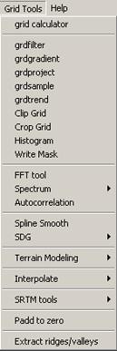 ·
grid
calculator – This is what it says.
It operates on loaded grids but you can also load more grids (as
long as they are GMT grids). When grids are loaded in
memory they will show up in the lower box area. Double-click on
a name to move it to the command area. The syntax used is that
of Matlab. This means that in principle any Matlab single
command that prduces a 2D array can be used to produce a new
image. eg: sin ( 10 * (repmat( linspace(-pi,pi,201),201,1).^2
+ repmat(linspace(-pi,pi,201)',1,201).^2) ) Notice that we
had to use repmat instead of meshgrid as we
usually would do because we need to produce the output array in
one single command like I said above.
·
grid
calculator – This is what it says.
It operates on loaded grids but you can also load more grids (as
long as they are GMT grids). When grids are loaded in
memory they will show up in the lower box area. Double-click on
a name to move it to the command area. The syntax used is that
of Matlab. This means that in principle any Matlab single
command that prduces a 2D array can be used to produce a new
image. eg: sin ( 10 * (repmat( linspace(-pi,pi,201),201,1).^2
+ repmat(linspace(-pi,pi,201)',1,201).^2) ) Notice that we
had to use repmat instead of meshgrid as we
usually would do because we need to produce the output array in
one single command like I said above.
-
·

-
grdfilter – will filter a grid in the time domain using a boxcar, cosine arch, gaussian, median, or mode filter and computing distances using Cartesian or Spherical geometries. The output can optionally be generated as a sub-region of the input and/or with a new increment. In this way, one may have "extra space" in the input data so that the edges will not be used and the output can be within one-half- width of the input edges. If the filter is low-pass, then the output may be less frequently sampled than the input.
· grdgradient – may be used to compute the directional derivative in a given direction, or the direction [and the magnitude] of the vector gradient of the data. Estimated values in the first/last row/column of output depend on boundary conditions.
· grdproject – Interface to grdproject (see Geographic calculator).
· grdsample – interpolates a grid to create a new grid with either: a new grid-spacing, or number of nodes, and perhaps also a new sub-region. Interpolation is bicubic [Default] or bilinear and uses boundary conditions. grdsample safely creates a fine mesh from a coarse one; the converse may suffer aliasing unless the data are filtered using grdfilter.
·
grdtrend
– reads a 2-D gridded file and fits a low-order
polynomial trend to these data by [optionally weighted]
least-squares. The trend surface is defined by:
m1 + m2*x + m3*y + m4*x*y + m5*x*x + m6*y*y
+ m7*x*x*x + m8*x*x*y + m9*x*y*y +
m10*y*y*y.
The user must specify n_model, the number
of model parameters to use; thus, 3 fits a bilinear
trend, 6 a quadratic surface, and so on.
Optionally, select to perform a robust fit. In this case, the
program will iteratively reweight the data based on a robust
scale estimate, in order to converge to a solution insensitive
to outliers. This may be handy when separating a "regional"
field from a "residual" which should have non-zero mean, such as
a local mountain on a regional surface. If data file has values
set to NaN, these will be ignored during fitting; if output
files are written, these will also have NaN in the same
locations.
· Clip grid – This corresponds to an interactive version of the grdclip GMT program. Shortly, values above "Above value" or below "Below value" are set to a desired value (including NaNs).
· Crop Grid – On images derived from grids, left click, drag and left click again. The rectangle thus defined is used to extract a subset of the original grid. This corresponds to an interactive version of the grdcut GMT program with the advantage that you will not fall onto the grips of the "Ivan the Terrible" (I mean the despairing message: GMT ERROR: (x_max-x_min) must equal (NX + eps) * x_inc), where NX is an integer and |eps| <= 0.0001). Note, this is a crude and poorly controlled way of doing a cropping operation. The best way is to draw a rectangle on the image. Calmly decide on its size and position (or conversely, on its limits) and than inquire its properties (by a right-click on the rectangle borders) for “Crop Tools -> Crop Grid”.
· Histogram – Compute an histogram of the z (grid) values. User is prompted to enter the histogram bin width. Note, this option is also available for rectangular ROIs.
· Write mask – With grids that contain NaNs it possible to write a mask grid in which the non NaNs will be replaced by the user entered value (e.g. 1).
· Spectrum – Compute either the log10 power or the amplitude spectrum. Note1, I am normalizing the FFT output by dividing by n_rows x n_columns. Note2, before FFTing the grid is cosine tapered to the extended dimension that better suits the two conditions: 1, the extended grid is at least 20% larger in both dimensions; 2, only “good FFT numbers” (with prime factors <= 5) are retained. Note3, this option is also available for rectangular ROIs.
· Autocorrelation – Compute the grid autocorrelation (it uses FFT). Note, this option is also available for rectangular ROIs.
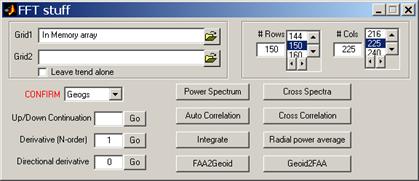
· FFT tool – This tool reproduces most of the functionalities of the grdfft GMT program (except filtering and the chaining of operations) and adds it some others. Namely the Cross Spectra and Cross Correlation. It is, however, entirely programmed in Matlab. That means double precision computations and potentially very large memory consumption.
· Spline Smooth – Uses cubic splines to smooth a grid. The important step in smoothing is the value of smoothing parameter. The smoothing parameter (p) determines the relative weight you would like to place on the contradictory demands of having f be smooth vs having f be close to the data. For p = 0, f is the least-squares straight line fit to the data, while, at the other extreme, i.e., for p = 1, f is the variational, or ‘natural’ cubic spline interpolant. As p moves from 0 to 1, the smoothing spline changes from one extreme to the other. The interesting range for p is often near 1/(1+h^3/6), with h the average spacing of the data sites, and it is in this range that the default value for p is chosen. For uniformly spaced data, one would expect a close following of the data for p = 1/(1+h^3/60) and some satisfactory smoothing for p = 1/(1+h^3/0.6). You can input a p > 1, but this leads to a smoothing spline even rougher than the variational cubic spline interpolant.
· SDG – SDG stands for Second Derivative in direction of Gradient. It is a very interesting operator, particularly to people working in the UNCLOS margins extension program. Shortly, it is the UN recommended algorithm to determine the Foot Of continental Slope (FOS). Even if you don’t know what I’m talking about, this operator worth trial because it has the ability to reveal very concealed trends in your data. It also depends on the smoothing parameter p as the previous option.
· Terrain modelling – In this section, the slope (either in degrees or percentage), aspect (that is the azimuth of the slope) and first and second directional derivatives of geographical referenced grids can be computed.
· Interpolate – Interpolate scattered x,y,z triplets into a regular grid array. Available options are GMT's surface and nearneighbor methods. Consult the corresponding GMT man pages for any droughts regarding these methods. Use should be obvious for anyone who knows what he/she is are trying to do.
·
SRTM
tools – 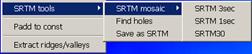 With the SRTM
mosaic tool you can draw a rectangle and select an interest
region. Right click on the rectangle and choose mesh.
This will draw yellow quadrangles corresponding to possible SRTM
tiles. Now a mouse click on each individual square will search
on the previously selected working directory for existing SRTM
With the SRTM
mosaic tool you can draw a rectangle and select an interest
region. Right click on the rectangle and choose mesh.
This will draw yellow quadrangles corresponding to possible SRTM
tiles. Now a mouse click on each individual square will search
on the previously selected working directory for existing SRTM 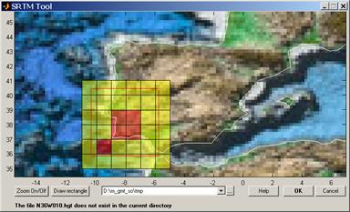 files (that may be .zip or .gz). If the matching file does exist
the square will turn red, if it doesn’t a warning message is
displayed during a second and the square will return to yellow.
Note, “mosaicing” is only possible with SRTM1 and 3 arc seconds
files. However, this tool is also handy for loading SRTM30+
files where it provides a nice graphical way of selecting the
tile of interest. The find holes option will
automatically detect regions of no data values (holes) and draw
rectangles around them. Right click on those rectangles and
select the options under crop tools to fill the holes. At
the end the processed file may be saved back into the SRTM
format. Note, saving back to SRTM is possible only for the 3 arc
seconds files.
files (that may be .zip or .gz). If the matching file does exist
the square will turn red, if it doesn’t a warning message is
displayed during a second and the square will return to yellow.
Note, “mosaicing” is only possible with SRTM1 and 3 arc seconds
files. However, this tool is also handy for loading SRTM30+
files where it provides a nice graphical way of selecting the
tile of interest. The find holes option will
automatically detect regions of no data values (holes) and draw
rectangles around them. Right click on those rectangles and
select the options under crop tools to fill the holes. At
the end the processed file may be saved back into the SRTM
format. Note, saving back to SRTM is possible only for the 3 arc
seconds files.
· Padd to zero – Cosine taper the grid to zero. The user is prompted for the extension number of rows/columns. This a useful option to pre-process bathymetry and elastic deformation grids before doing tsunami propagations because it highly reduces the annoying (and false) grid edge reflections.
· Extract ridge/valleys – Again this is more an intention than a true useful tool. While it works reasonably well (but be careful and do not abuse with grid size) in extracting ridges (only working mode) the problem is that the ppa (ref) algorithm used outputs the crest lines as a sequence of non-contiguous two point lines segments. This makes it impossible to treat them as polylines.
“Hidden” options
Mirone still has a LOT more of options that are not ranged in menus, for the simple reason that there is no way to do it without complicating enormously the graphical interface. Instead they only show up when the situations make it appropriate and than they are accessible with a mouse right-click on a graphical element. For example, polygons drawn on a grid derived grid let you do a median filter that is applied only to the grid nodes inside the polygon. I wrote this option at sea when I wanted to get rid of those awful effects that result on the overlap of contiguous swaths on multi-beam surveys. On the other hand, if the polygon is an exact rectangle you can do FFT like operations. Another example is given by right-clicking on the axes coordinates. If the grid is in geographical coordinates, you can than select among several different ways of displaying degrees (eg, dd.xxxx or dd:mm:ss). Furthermore, if you decide to save a line into an ascii file, the x,y coordinates will be formatted in the same way as the selected coordinate display. I hope that this will be appreciated by those of you who know what is getting a way points, picked on a computer screen in deg.xx, go up to the ship’s bridge and listen the Captain (or whoever is driving the ship that dawn) tell you “Can’t you give me those way points in degrees and minutes?”
Installation
First, you have to install GMT. This as difficult as to download the setup HERE and click next to all options. Mirone is distributed in both source code and a Windows compiled stand-alone version. Incredibly as it might seam, the source code version is faster than its compiled counterpart. The condition is that you have Matlab 6.5 version (or higher). To run it from Matlab, unzip the source code to wherever directory you want. Within Matlab, change to that directory and write "mirone" (without the ") on the command prompt. This, however, is a wasteful way of doing things. The point is that Matlab with its Java interface consumes a lot of computer memory and has a lousy memory management capacity (I mean, and sustain; it doesn’t free all memory after use). A better way is if you start Matlab with the -nojvm option. This saves a lot of computer resources. See the instructions on the startup.m file that you find on the Mirone’s installation directory for how to create a desktop icon to do this automatically. Nothing of the previously said implies dependency to a particular Operating System, so Mirone should run equally in Windows or Unix/Linux or Mac OS X. However, in order to run it in non-Windows platforms, a bunch of mex files have to be compiled for that system. The GDAL library it self must be installed. The mex files can be built from the files that are installed under the "mex" directory of the root’s Mirone directory. Regarding instructions on how to compile them under other OSs the most I can help you right now is, see the make_mexs.m file and try to adapt it to your environment.
On the other hand, the compiled version works only in Windows. It is provided as a setup where you only have to say "yes" to most of the questions. At the end you will have one more icon on your desktop. If, however, you decided to not accept the proposed destination directory, you will have to edit the mirone.bat in order that the PATH variable reflects where you did install the program. If you don’t do this correctly, the program won’t work by the simple reason that it doesn’t know where it is. The symptom of this problem shows up in the form a little window saying that it cannot find a dll. A final note to users that like to install their programs in directories with blanks on their names (like “Program Files”). Simply DO NOT DO IT, first it is a very bad habit (I know that B. Gaitas Inc induce you to do so) but regarding Mirone and GMT you will very soon run into troubles.