Fine picking of a magnetic isochron
Describe how to do pickings of a magnetic isochron from a magnetic anomaly grid previously reduced to the pole.
Load the magnetic anomaly grid and display it with a nice 'magnetic color palette' plus shading illumination
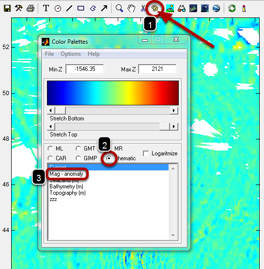
This example uses one magnetic anomaly grid centered on the North Central Mid-Atlantic-Ridge. After loading the grid we will display it with a color scale appropriate for magnetic anomalies. We do that by bringing up the Color Palette tool (1), select the Thematic group in (2) and finally choosing the "Mag - anomaly" in (3)
Shade illuminate with the Lambertian algorithm
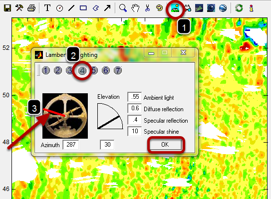
Load the Shade illumination tool (1), select the method 4 (2) and click and drag the red line so that it look like the in (3) and at end hit the OK button
The shaded illuminated magnetic anomaly
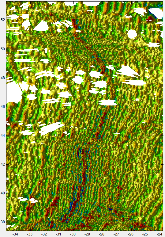
This is how it looks after the steps described above. In the next figure we will display a zoom of the south part.
Extract a profile from grid
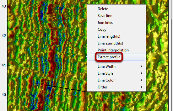
Use the "Draw line" button on the menu bar to plot one line like in the figure. Right-click on the line to bring up the menu and select the "Extract profile". This will create the next figure.
Magnetic profile
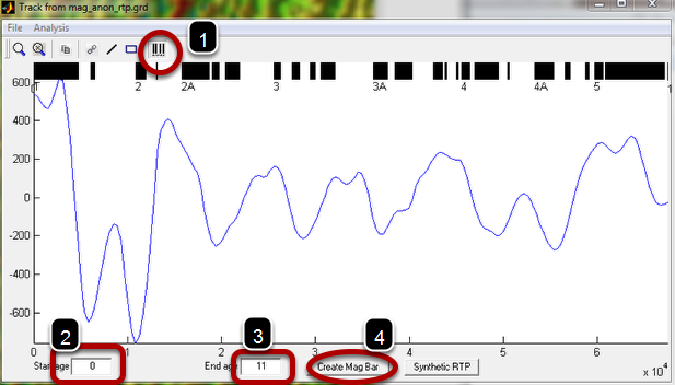
Hit the bar code icon on (1) to make visible the edit boxes (2) and (3). The use of them is to enter the start and end age of the magnetic profile. Because we started the magnetic profile on the ridge we know its age is 0 Ma, and since I know the place, I know the end is a bit after the end of anomaly 5 so we will use an age of 11 Ma (the value doesn't need to be exact anyway). Hit the "Create Mag Bar" button (4) and the "magnetic bar code" (Geomagnetic reversal time scale) is plotted on top. Because this a nicely behaved magnetic profile it's easy to pick the magnetic isochrons and we have the time scale to help us recognizing which is which.
Pick anomalies and plot them on the mag grid image
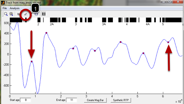
Click on the link icon (1) to start picking the anomalies. the cursor turns into a cross and every left-click adds one point. To stop make a right-click. Because the magnetic anomaly used in this example is Reduced To the Pole (RTP) and center of the anomalies correspond to the age of their mid period. But what is more interesting here is that the picks on this image were transported also to the anomaly image. See
Point clicks on their exact locations
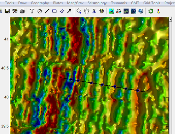
Anomaly pickings of the sequence C2, C2A, C3, C3A, C4, C4A and C5 isochrons. Now the hard work is to repeat this procedure for many profiles, on both sides of the ridge, so that we can have a as much as possible complete set of isochrons identifications that can be used to compute Euler poles to do kinematic reconstructions. But that is the subject of another lesson.